Solving Facility Location Problems

Introduction
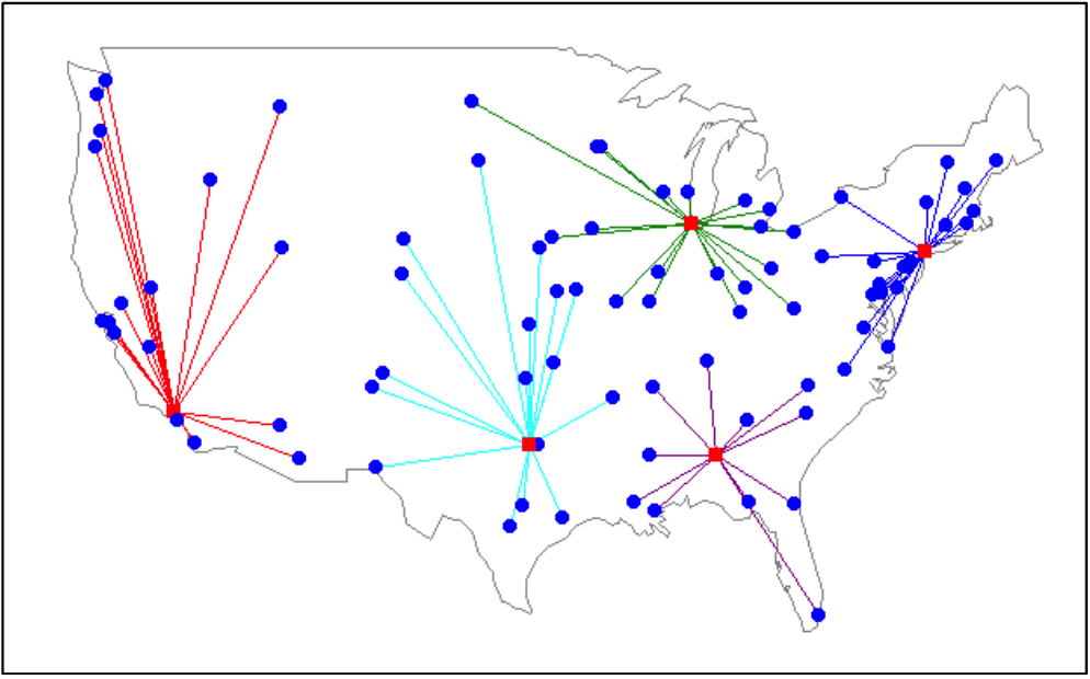
Where to set up factories and workshops is one of the typical problems of industrial engineering. This type of model usually takes into account issues such as demand, shipping costs and inventory costs to find the most suitable location to set up facilities.
Therefore, this article applies three common models to solve facility location problems:
1. Uncapacitated fixed-charge location problem(UFLP):
Minimize fixed + transportation cost
2. Set covering location problem(SCLP):
Minimize number of facilities
3. Maximum covering location problem(MCLP):
Maximize covered demands
Language/ Tool/ Package
Python
- gurobipy: The Gurobi Optimizer is a mathematical optimization software library for solving mixed-integer linear and quadratic optimization problems.
- pandas: open source data analysis and manipulation tool
- itertools: this module implements a number of iterator building blocks inspired by constructs from APL, Haskell, and SML.
Background Information
1. Customer
Data for a 10- node demands, fixed cost and location (express by x, y)
| Index | x | y | Demand | Fixed Cost |
|---|---|---|---|---|
| 1 | 0.2 | 0.1 | 60 | 200 |
| 2 | 0.9 | 0.7 | 27 | 200 |
| 3 | 0.2 | 0.4 | 29 | 200 |
| 4 | 0.9 | 0.2 | 26 | 200 |
| 5 | 0.5 | 0.9 | 33 | 200 |
| 6 | 0.6 | 0.3 | 15 | 200 |
| 7 | 0.8 | 0.4 | 17 | 200 |
| 8 | 0.5 | 0.3 | 97 | 200 |
| 9 | 0.3 | 0.6 | 97 | 200 |
| 10 | 0.2 | 0.6 | 19 | 200 |

2. Distance:
Distance is computed by Euclidean distance between the nodes.
| Facilities | 1 | 2 | 3 | 4 | 5 | 6 | 7 | 8 | 9 | 10 |
|---|---|---|---|---|---|---|---|---|---|---|
| 1 | 0.0000 | 9.2195 | 3.0000 | 7.0711 | 8.5440 | 4.4721 | 6.7082 | 3.6056 | 5.0990 | 5.0000 |
| 2 | 9.2195 | 0.0000 | 7.6158 | 5.0000 | 4.4721 | 5.0000 | 3.1623 | 5.6569 | 6.0828 | 7.0711 |
| 3 | 3.0000 | 7.6158 | 0.0000 | 7.2801 | 5.8310 | 4.1231 | 6.0000 | 3.1623 | 2.2361 | 2.0000 |
| 4 | 7.0711 | 5.0000 | 7.2801 | 0.0000 | 8.0623 | 3.1623 | 2.2361 | 4.1231 | 7.2111 | 8.0623 |
| 5 | 8.5440 | 4.4721 | 5.8310 | 8.0623 | 0.0000 | 6.0828 | 5.8310 | 6.0000 | 3.6056 | 4.2426 |
| 6 | 4.4721 | 5.0000 | 4.1231 | 3.1623 | 6.0828 | 0.0000 | 2.2361 | 1.0000 | 4.2426 | 5.0000 |
| 7 | 6.7082 | 3.1623 | 6.0000 | 2.2361 | 5.8310 | 2.2361 | 0.0000 | 3.1623 | 5.3852 | 6.3246 |
| 8 | 3.6056 | 5.6569 | 3.1623 | 4.1231 | 6.0000 | 1.0000 | 3.1623 | 0.0000 | 3.6056 | 4.2426 |
| 9 | 5.0990 | 6.0828 | 2.2361 | 7.2111 | 3.6056 | 4.2426 | 5.3852 | 3.6056 | 0.0000 | 1.0000 |
| 10 | 5.0000 | 7.0711 | 2.0000 | 8.0623 | 4.2426 | 5.0000 | 6.3246 | 4.2426 | 1.0000 | 0.0000 |
Uncapacitated Fixed-charge Location Problem (UFLP)
- Minimize fixed + transportation cost
Example:
The background information contains nodes located on the unit square and I = J. The background information lists the x- and y-coordinates, demands hi, and fixed costs fj for each node, as well as the transportation cost cij between each pair of nodes i and j. Transportation costs equal 10 times the Euclidean distance between the nodes. All fixed costs equal 200.
Solution Approach:
Decision variables:
cartesian_prod = list(product(range(0, 10), range(0, 10)))
cust = m.addVars(cartesian_prod, lb = 0 ,vtype = GRB.CONTINUOUS, name='cust')
Objection:
m.setObjective(gp.quicksum(df_demand[customer] * shipping_cost[customer, facility] * cust[customer, facility] for customer in range(0, 10) for facility in range(0, len(fact))) + gp.quicksum(fact[facility] for facility in range(0, len(fact))) * 200 , GRB.MINIMIZE)
Constraints:
m.addConstrs((gp.quicksum(cust[(customer, facility)] for facility in range(0, 10)) == 1 for customer in range(0, 10)), name='Demand')

m.addConstrs((cust[customer, facility] <= fact[facility] for customer, facility in cartesian_prod), name='Setup2ship')
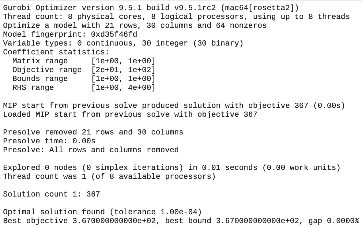
Results:

Code
Set Covering Location Problem (SCLP)
- Minimize number of facilities
Example:
Using the data from background information, solve the SCLP exactly by implementing it in the modeling language with a MIP solver. Set the fixed cost of every facility equal to 1. Assume that facility j covers customer i if cij ≤ 2.5. Report the optimal locations.
Solution Approach:
Decision variables:
fact = m.addVars(10, vtype = GRB.BINARY, name='fact')
Objection:
obj = gp.quicksum(f * fact[facility] for facility in range(0, 10))
m.setObjective(obj, GRB.MINIMIZE)
Constraints:
m.addConstrs((gp.quicksum(aij[(customer, facility)] * fact[facility] for facility in range(0, 10)) >= 1 for customer in range(0, 10)), name='coverage')
Results:

Code
Maximum covering location problem (MCLP)
- Maximize covered demands
Example:
Using the data from background information, solve the MCLP exactly by implementing it in the modeling language with a MIP solver. Set p = 4. Assume that facility j covers customer i if cij ≤ 2.5.
Report the optimal locations and the total number of demands covered.
Solution Approach:
Decision variables:
fact = m.addVars(10, vtype = GRB.BINARY, name='fact')
Objection:
obj = gp.quicksum(f * fact[facility] for facility in range(0, 10))
m.setObjective(obj, GRB.MINIMIZE)
Constraints:
m.addConstrs((gp.quicksum(aij[(customer, facility)] * fact[facility] for facility in range(0, 10)) >= 1 for customer in range(0, 10)), name='coverage')
Results:
